By: Naitik Chheda
Abstract
This study employs an agent‐based simulation framework to compare the performance of diverse trading strategies across five distinct market regimes: sideways, high-volatility, euphoria, crash, and cyclical. Synthetic market data are generated using a combination of Ornstein–Uhlenbeck processes, geometric Brownian motion with drift, and sinusoidal models with noise to emulate real-world market conditions. Heterogeneous agents, each implementing a specific trading heuristic (Contrarian, Optimist, Trend Follower, Swing Trader, and Fundamentalist), operate on this simulated market. Performance is evaluated via a composite score that balances return, volatility, and drawdown. The results demonstrate regime-specific strengths: while trend-following approaches mitigate losses during downturns, fundamental and contrarian strategies excel in volatile environments. The findings suggest that aligning trading strategies with prevailing market regimes can enhance risk-adjusted returns, thereby providing insights into adaptive trading in complex financial systems.
1. Introduction
Financial markets are inherently complex and dynamic systems where the interplay between market regimes and trading strategies can determine overall performance. Over the past few decades, agent-based modeling (ABM) has emerged as a powerful tool to simulate and analyze the behavior of heterogeneous market participants under varying conditions. Unlike traditional models that often rely on equilibrium assumptions or representative agents, ABMs capture individual decision rules and interactions, thereby offering a bottom-up perspective on market phenomena.
Despite extensive literature on technical and fundamental analysis, the effectiveness of distinct trading strategies remains highly sensitive to market conditions. For instance, empirical studies and simulation-based analyses (Cont, 2001 & LeBaron, 2006) indicate that market volatility and regime shifts can profoundly affect the risk–return tradeoff of different strategies. This paper builds on these insights by creating a controlled simulation environment where five trading heuristics are tested against five synthetic market regimes.
This research demonstrates that the performance of trading strategies is significantly influenced by market regime conditions. By aligning specific strategies, such as fundamental analysis and mean-reversion techniques, with corresponding regimes, traders can achieve superior risk-adjusted returns compared to a one-size-fits-all approach.
2. Literature Review
2.1 Agent‐Based Models in Financial Markets
Agent‐based computational economics has become a well‐established methodology for exploring financial market dynamics. Early work by Arthur et al. (1997) and subsequent reviews by LeBaron (2006) and Tesfatsion (2006) demonstrate how ABMs can capture the emergent phenomena, such as fat-tailed return distributions, volatility clustering, and regime shifts, that traditional equilibrium models cannot adequately explain. These studies highlight that by simulating interactions among heterogeneous, boundedly rational agents, ABMs are uniquely suited to replicate microstructural market behaviors and to test how individual rules translate into macro-level outcomes.
2.2 Synthetic Market Data Generation
Realistic simulation of market conditions requires generating synthetic data that mirror the statistical properties of actual markets. Researchers have employed stochastic processes, such as the Ornstein–Uhlenbeck process for mean reversion and geometric Brownian motion for trending behaviors, to simulate distinct market regimes (e.g., sideways, high volatility, euphoria, crash, and cyclical markets). This approach is supported by studies that compare simulated data with historical records, confirming that well-calibrated synthetic data can reproduce key stylized facts (Cont, 2001) and serve as an effective test bed for evaluating trading strategies.
2.3 Heterogeneous Trading Strategies and Behavioral Agents
A critical aspect of our research is the exploration of multiple trading strategies executed by heterogeneous agents. The literature on technical trading and behavioral finance documents that diverse heuristics, such as contrarian (mean-reversion), trend-following, buy-and-hold (optimistic), swing trading, and fundamental analysis, can lead to markedly different performance under varying market conditions. For example, Chiarella (2002) discusses the efficacy of moving-average strategies under different volatility regimes, while fundamental approaches have been noted for their robustness in volatile markets. ABM studies further show that incorporating small random variations in decision parameters helps capture real-world heterogeneity among traders, an approach that strengthens the realism of simulated markets and supports the analysis of regime-dependent strategy performance.
2.4 Evaluation Metrics and Risk Management
Evaluating strategy performance in simulated markets requires metrics that capture both return and risk. Prior research has combined measures such as total return, return volatility, and maximum drawdown to form composite scores—metrics that reward high returns but penalize excessive risk. This composite approach aligns with risk management practices in quantitative finance (Derman, 2016) and provides a more nuanced evaluation than return measures alone. By benchmarking simulated strategies across different market regimes, these metrics facilitate a robust analysis of how trading rules perform under both favorable and adverse conditions.
3. Methodology
The approach presented herein integrates stochastic data generation with an agent-based simulation framework to investigate the performance of various trading strategies across different market regimes. Synthetic market data are produced using established stochastic processes, and heterogeneous agents are modeled to follow distinct trading heuristics. The simulation yields time series data for portfolio values, which are subsequently analyzed through quantitative performance metrics and visualizations. To put simply, the method creates simulated market data using proven mathematical models, then tests how different types of trading rules perform in these markets, and finally compares their results.
3.1 Data Creation and Market Simulation
The synthetic market data are generated to represent five distinct market regimes: Sideways Market, High-Volatility Market, Euphoria Regime, Crash Regime, and Cyclical Market. For each regime, specific stochastic processes are employed.
In the Sideways Market, asset prices are modeled using an Ornstein–Uhlenbeck (OU) process with a subtle upward drift. The dynamics are described by
dS(t)=θ(S0−S(t))dt+σ dW(t)+μsidewaysdt
where S(t) denotes the asset price at time t, S0 is the initial (and long-term mean) price, θ is the rate of mean reversion, σ is the volatility, μsideways is a small constant drift, and dW(t) is the increment of a Wiener process. Simply put, this equation means that prices tend to hover around a central value (with small random ups and downs) while slowly increasing over time, a behavior seen in real markets (Cont, 2001) and can be seen in the figure below.

Figure 1 - Sideways Market
For the High-Volatility Market, rather than using a standard geometric Brownian motion, which can result in extreme values over long horizons, the logarithm of the asset price is modeled via a mean-reverting OU process:
dX(t)=θ(μ−X(t))dt+σdW(t), S(t)=exp{X(t)}
The parameter μ is set as
μ=ln(S0)−σ24
so that the stationary expectation of S(t) is approximately S0 (Karatzas & Shreve, 1998). In essence, even though the prices fluctuate wildly, this method ensures they do not spiral out of control or drop to zero in the long run and can be seen in the figure below.
Figure 2 - High Volatility Market
The Euphoria Regime employs a geometric Brownian motion (GBM) with a positive drift:
dS(t)=μS(t)dt+σS(t) dW(t)
where μ > 0 and σ is set to moderate values so that a strong upward trend is produced. This creates a scenario where prices are consistently rising, as might be seen during a market boom and can be seen in the figure below.
Figure 3 - Euphoria Market
Conversely, the Crash Regime is generated by setting μ < 0 in the same GBM framework, producing a downward trend. Here, prices steadily fall, modeling a market downturn and can be seen in the figure below.
Figure 4 - Crash Market
The Cyclical Market is constructed by superimposing a deterministic sinusoidal function on a base price with additive Gaussian noise:
S(t)=S0+Asin(2tT)+ϵt
where A is the amplitude, T represents the period of the cycle, and ϵt is a normally distributed noise term. Basically, this means that prices go up and down in a regular, repeating pattern with some added noise, similar to seasonal effects or business cycles (Hsieh, 1991) and can be seen in the figure below.
Figure 5 - Cyclical Market
3.2 Agent Definitions and Trading Strategies
A multi-agent system is implemented, where each agent begins with an identical initial capital. Heterogeneity among agents is introduced through small random variations in key decision parameters. Five distinct strategies are used:
Contrarian Agent:
The Contrarian agent utilises mean-reversion by computing a moving average over a window of w timesteps:
MA(t)=1w i=t-wt-1 S(i)
A trade is initiated when the current price S(t) deviates from MA(t) by a margin δ. A buy signal is generated if
S(t)<MA(t) × (1−δ)
and a sell signal if
S(t)>MA(t) × (1+δ)
This means that if the price falls much below its recent average, the agent buys expecting it to return to normal, and if it rises much above, the agent sells. This mirrors the idea of “buy low, sell high.”
Optimist Agent:
This agent follows a simplistic buy-and-hold strategy by purchasing additional units of the asset whenever sufficient capital is available, anticipating continual upward price movement. In simpler terms, it keeps buying because it assumes that prices will keep going up.
Trend Follower Agent:
This strategy employs two moving averages, a short-term average MAs(t) computed over ws timesteps, and a long-term average MAl(t) computed over wl timesteps (with ws < wl). The momentum M(t) of the short-term average is also estimated:
M(t)=MAs(t)−MAs(t−1)
A buy signal is produced if
MAs(t)>MAl(t) and M(t)> δMAl(t)
while a sell signal is issued when
MAs(t)<MAl(t) and M(t)< -δMAl(t)
In other words, if the recent average price is above the long-term average and rising, the agent buys. On the other hand, if it is below and falling, the agent sells. This helps capture short-term trends effectively (Chiarella, 2002).
Swing Trader Agent:
Designed to capture cyclical fluctuations, this agent calculates the normalized position p(t)p(t)p(t) of the current price within a lookback window:
p(t)=S(t)−min{S(i):t−w≤i<t}max{S(i):t−w≤i<t}−min{S(i):t−w≤i<t}
With an additional momentum check, a buy signal is generated when p(t) is below a lower threshold and the price is beginning to rebound, while a sell signal is triggered when p(t) exceeds an upper threshold and the price starts to decline. This means that if the price is near its recent low and begins to rise, the agent buys, and if it is near its recent high and begins to drop, the agent sells.
Fundamentalist Agent:
The Fundamentalist agent assumes that each asset has an intrinsic value S*. Trading decisions are based on the difference between the current price S(t) and S*. A buy signal is generated if
S(t)< S* × (1−θf)
and a sell signal if
S(t)> S* × (1+θf)
Simply, if the price is much lower than what is believed to be its true value, the agent buys; if it is much higher, the agent sells (Graham & Dodd, 1934).
3.3 Simulation Process
The simulation operates in discrete timesteps. At each timestep, the asset price is determined by the appropriate market regime model. Each agent observes the current price and calculates a trading signal based on its strategy. If a buy signal is generated, the agent purchases one unit of the asset (provided that it has sufficient funds). Similarly, if a sell signal is issued, the agent sells one unit (subject to availability). The portfolio value of each agent is updated as
Portfolio(t)=Cash(t)+Stock(t)×S(t)
and recorded throughout the simulation.
3.2 Evaluation and Scores
After the simulation, the performance of each agent is evaluated using several key metrics. The total return is calculated as the final portfolio value relative to the initial capital. Volatility is measured as the standard deviation of the periodic returns, and the maximum drawdown is defined as the largest percentage decline from a peak portfolio value during the simulation. These metrics are combined into a composite score:
Composite Score=Return−Volatility−Max Drawdown
This score is designed to reward high returns while penalizing large fluctuations and deep losses.
4. Results
The simulated outcomes shed light on each strategy’s behavior and performance across a range of market conditions (Sideways, High Volatility, Euphoria, Crash, and Cyclical). The final outputs shown in the tables and figures (e.g., the average portfolio value plots over time and the heatmaps) collectively illustrate how different agent strategies fared. Key observations are summarized below.
4.1 Sideways Market
The average portfolio values in Figure 6 reveal that Contrarian and SwingTrader agents maintain portfolio values slightly above their initial levels, while the Optimist agent remains nearly flat. The TrendFollower agent exhibits small, negative performance, consistent with the notion that strict trend‐following often struggles in sideways conditions. The Fundamentalist ends up close to its starting value, demonstrating a conservative approach. The results shows that Contrarian has a positive composite score (0.0312), though quite small, while Optimist’s score is −0.1232 and TrendFollower’s is −0.0106.
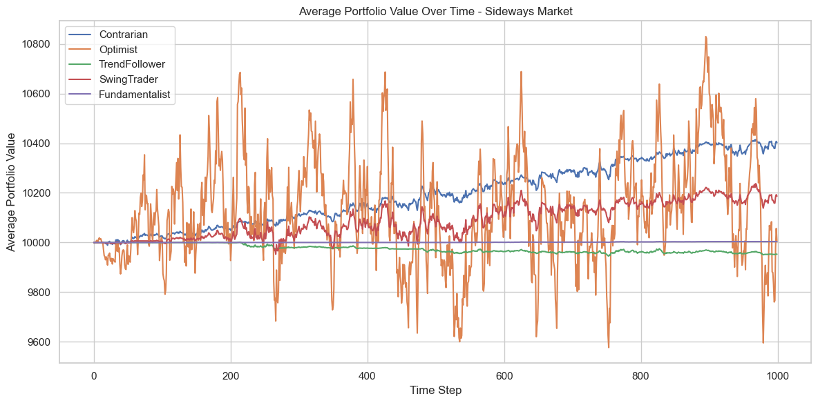
Figure 6 - Sideways Market Portfolios
4.2 High-Volatility Market
Figure 7 shows dramatic fluctuations in average portfolio values, with the Fundamentalist and Contrarian strategies at times surging to exceptionally high portfolio values. The heatmap of final portfolio values confirms that the Fundamentalist strategy averages around 60,000, compared to Contrarian’s 45,000, both being significantly higher than other strategies. This outperformance likely stems from the agent systematically buying the asset when it is underpriced relative to a perceived fundamental value and selling when overpriced, capitalizing on large swings. The summary composite scores also underscore this distinction: Fundamentalist reaches 4.3999 while Contrarian is 2.6472, both outshining the other approaches in this regime.
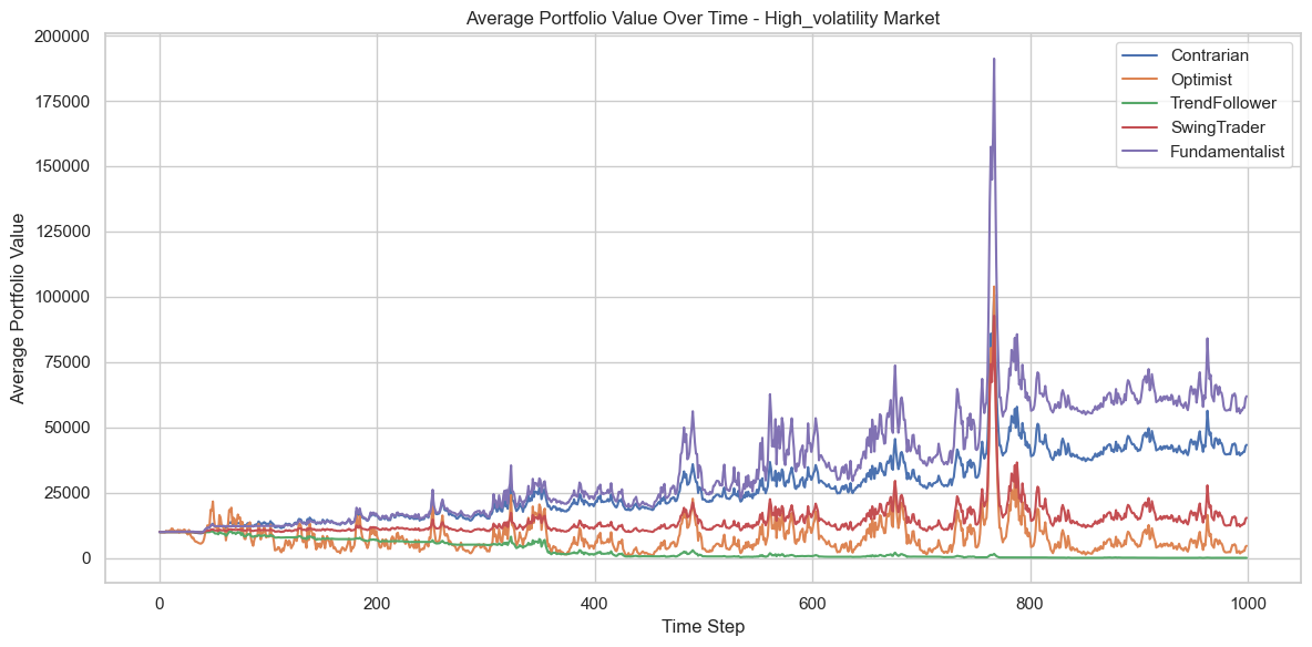
Figure 7 - High-Volatility Market Portfolios
4.3 Euphoria Market
As seen in Figure 8, Optimist quickly becomes dominant, reaching an average portfolio value of over 30,000 by the final timestep. The TrendFollower agent also does relatively well, ending with a final value close to 20,000. The Contrarian and SwingTrader remain behind, although Contrarian achieves a modest increase over the initial capital. The final composite scores in the euphoria setting underscore this pattern: Optimist attains 2.0290, while TrendFollower’s is 0.8249. Contrarian, SwingTrader, and Fundamentalist lag behind with respective scores of 0.1614, 0.0814, and 0.0229.
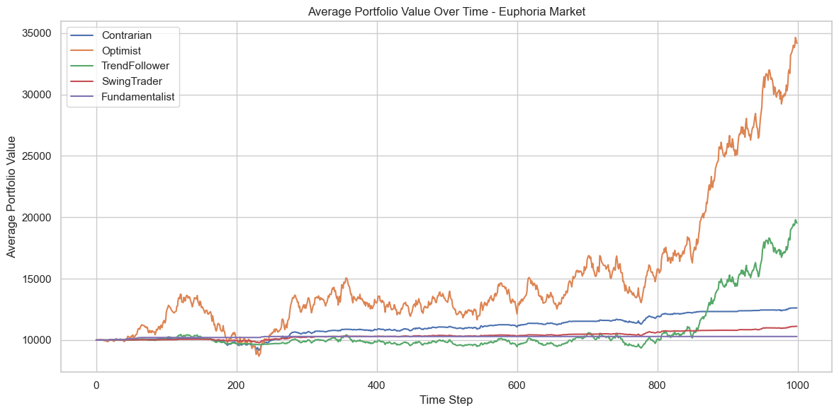
Figure 8 - Euphoric Market Portfolios
4.4 Crash Market
In a sustained market downturn (Figure 9), TrendFollower outperforms most others. The average portfolio value for TrendFollower declines more slowly, finishing around 5,000–6,000, while Contrarian and Fundamentalist end the simulation in the 3,000–5,000 range on average. Optimist is the hardest hit, consistently buying into a falling market and ultimately ending below 1,000. The composite scores show a negative but relatively smaller loss for TrendFollower (−0.0783), whereas Contrarian is −0.9773 and Optimist −1.8863. This result aligns with the expectation that momentum‐based strategies can switch to a “sell” signal in a declining market, thus preserving more capital.
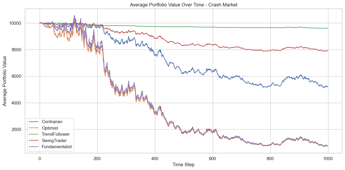
Figure 9 - Crash Market Portfolios
4.5 Cyclical Market
In Figure 10, Fundamentalist has the highest average portfolio value by the end (~15,000), with Contrarian and SwingTrader oscillating around 10,000–11,000. The Optimist agent remains lower, around 9,000–10,000, despite benefiting briefly when the cycle’s upward swings coincide with repeated buys. TrendFollower lags slightly due to the rapid reversals of cyclical conditions. The composite scores confirm these patterns: Fundamentalist is 0.4880, Contrarian 0.2147, and TrendFollower −0.3148.
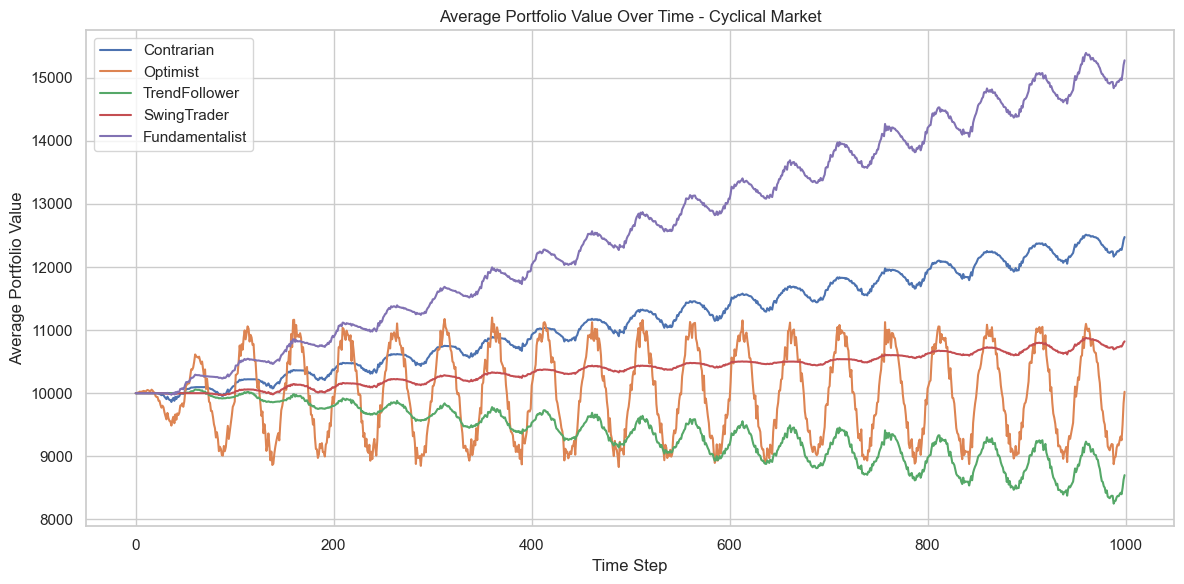
Figure 10 - Cyclical Market Portfolios
4.6 Composite Scores and Final Outcomes
The heatmaps summarizing the final portfolio values (Figure 11) and composite scores (Figure 12) show that each strategy exhibits distinct regimes of outperformance:
-
Fundamentalist achieves the highest global composite score of 0.6058, reflecting robust performance in high‐volatility and cyclical markets.
-
Contrarian follows with a global composite score of 0.4154, bolstered by high‐volatility gains and decent outcomes in sideways and cyclical environments.
-
Optimist scores −0.4079, enjoying strong gains in euphoria but suffering heavily in crash and high‐volatility regimes.
-
TrendFollower outperforms in the crash regime, but it exhibits negative or modestly positive returns in others, yielding an overall score of −0.3431.
-
SwingTrader hovers at −0.1408, performing moderately well in certain conditions (sideways, cyclical) but lacking the standout success of Contrarian or Fundamentalist in high‐volatility scenarios.
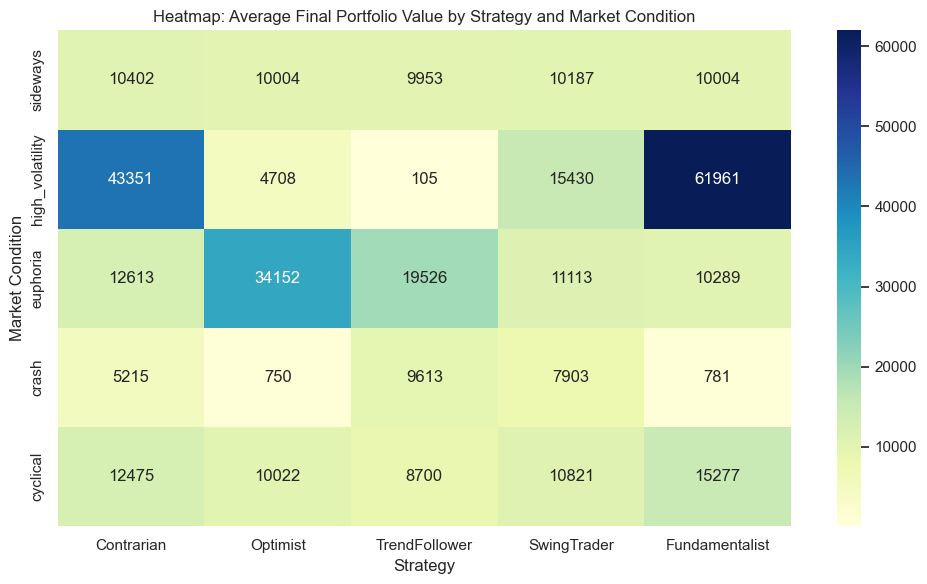
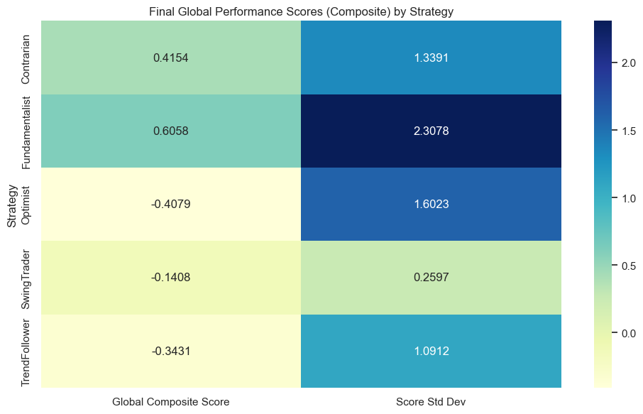
Figure 11 - Final Portfolio Values Figure 12 - Final Performance Scores
5. Analysis and Discussion
The findings point to several crucial insights:
5.1 Role of Market Regime on Strategy Success
As anticipated in previous studies (LeBaron, 2006), trading strategies are highly sensitive to the underlying market conditions. In a crash, momentum‐based approaches (TrendFollower) limit losses better than optimistic buy‐and‐hold. Conversely, during euphoria, Optimist far outpaces more cautious strategies, reflecting the benefit of relentless buying in a generally rising market.
5.2 Mean-Reversion vs Fundamental Anchors
In high‐volatility scenarios, Contrarian and Fundamentalist approaches excel by exploiting significant price swings. The Fundamentalist agent’s consistent comparison to a theoretical “true value” allows it to systematically buy undervalued assets and sell overvalued ones. Contrarian logic (buy low, sell high based on recent prices) yields a similar advantage but depends more on short‐term reversion than long‐term intrinsic value. Both agents illustrate that significant price fluctuations can be leveraged effectively if a strategy can identify perceived mispricings.
5.3 Implications for Risk Management
The composite scores integrate return, volatility, and drawdown, revealing that robust performance is not solely about maximizing returns but also about controlling risk. For instance, while Optimist experiences large gains in euphoria, its overall score is negative because sustained drawdowns in crash and high‐volatility regimes overshadow those gains. In practice, risk‐conscious traders may prefer strategies that sacrifice some upside potential for greater capital preservation (Derman, 2016).
5.4 Validity and Relevance of the Results
Although based on simulated markets rather than real‐world data, these findings are consistent with well‐documented phenomena. For instance, the difficulties of buy‐and‐hold strategies in a crash reflect real‐life drawdowns seen in crises such as 2008–2009. Mean‐reversion and fundamental approaches are known to have pronounced success in markets with large price swings (Poterba & Summers, 1988). While no simulation can perfectly replicate real financial dynamics, the alignment with known patterns lends credibility to the findings.
6. Conclusion
This research presents an agent‐based simulation framework incorporating multiple trading heuristics and distinct market regimes to examine strategy performance under varying conditions. The results demonstrate that each agent thrives in certain environments and struggles in others. In high‐volatility scenarios, Contrarian and Fundamentalist agents systematically exploit price swings to generate higher returns, whereas Optimist significantly outperforms in bullish (euphoria) markets yet suffers heavy losses in crashes. TrendFollower and SwingTrader perform moderately well in certain phases but rarely match the peak outcomes of specialized strategies.
Overall, Fundamentalist emerges with the highest composite score across all regimes, indicating robust risk‐adjusted returns over longer horizons. Meanwhile, Contrarian ranks second, pointing to the efficacy of mean‐reversion approaches in turbulent markets. The analysis underscores that market structure and agent strategy must be aligned; a single all‐purpose strategy does not emerge. These findings reinforce the principle that no one strategy universally dominates and that adaptive, condition‐specific approaches may offer better longevity in unpredictable, real‐world financial markets.
7. References
Arthur, W. B., Holland, J. H., LeBaron, B. D., Palmer, R. G., & Tayler, P. (1997). Asset Pricing Under Endogenous Expectations in an Artificial Stock Market. SSRN Electronic Journal. https://doi.org/10.2139/ssrn.2252
Chiarella, C., He, C., & He, X. T. (2024). Heterogeneous Beliefs, Risk and Learning in a Simple Asset Pricing Model. Computational Economics, 19(1), 95–132. https://econpapers.repec.org/article/kapcompec/v_3a19_3ay_3a2002_3ai_3a1_3ap_3a95-132.htm
Cont, R. (2001). Empirical properties of asset returns: stylized facts and statistical issues. Quantitative Finance, 1(2), 223–236. https://doi.org/10.1080/713665670
Derman, E., & Miller, M. B. (2016). The Volatility Smile. https://doi.org/10.1002/9781119289258
Graham, B., & Dodd, D. L. (1934). Security analysis. Mcgraw-Hill.
Hsieh, D. (1991). Chaos and Nonlinear Dynamics: Application to Financial Markets. The Journal of Finance, 46(5), 1839–1877. https://doi.org/10.1111/j.1540-6261.1991.tb04646.x
Kamyab, Y., & Hadzikadic, H. (n.d.). AN AGENT-BASED STUDY OF HERDING RELATIONSHIPS WITH FINANCIAL MARKETS PHENOMENA. Retrieved February 2, 2025, from https://informs-sim.org/wsc17papers/includes/files/093.pdf
Karatzas, I., & Shreve, S. E. (1998). Brownian Motion and Stochastic Calculus. In Graduate Texts in Mathematics. Springer New York. https://doi.org/10.1007/978-1-4612-0949-2
LeBaron, B. (2006). Agent-based Computational Finance. Handbook of Computational Economics, 1187–1233. https://doi.org/10.1016/s1574-0021(05)02024-1
Liu, X., Res, M., & Brooks, R. (n.d.). Replicating agent-based simulation models of herding in financial markets. https://eprints.lancs.ac.uk/id/eprint/162652/1/2021xinliuphd.pdf
Llacay, B., & Peffer, G. (2017). Using realistic trading strategies in an agent-based stock market model. Computational and Mathematical Organization Theory, 24(3), 308–350. https://doi.org/10.1007/s10588-017-9258-0
Poterba, J. M., & Summers, L. H. (1988). Mean reversion in stock prices. Journal of Financial Economics, 22(1), 27–59. https://doi.org/10.1016/0304-405x(88)90021-9
Tesfatsion, L. (2006). Agent-Based Computational Economics: A Constructive Approach to Economic Theory. Handbook of Computational Economics, 2, 831–880. https://ideas.repec.org/h/eee/hecchp/2-16.html